Time evolution
Time evolution with paulistrings.py is performed in the Heisenberg picture. This is because pure states are rank-1 density matrices, and low-rank density matrices cannot be efficiently encoded as a sum of Pauli strings.
The advantage of working with Pauli strings is that noisy systems can be efficiently simulated in this representation ([Schuster 2024](https://arxiv.org/abs/2407.12768)). Depolarizing noise causes long strings to decay, making simulations tractable by combining noise with truncation.
Let’s time-evolve the operator \(Z_1\) in the chaotic spin chain:
First, we construct the Hamiltonian:
import paulistrings as ps
def chaotic_chain(N):
    H = ps.Operator(N)
    # XX interactions
    for j in range(N - 1):
        H += "X", j, "X", j + 1
    H += "X", 0, "X", N - 1  # close the chain (periodic)
    # fields
    for j in range(N):
        H += -1.05, "Z", j
        H += 0.5, "X", j
    return H
We initialize a Hamiltonian and the \(Z_1\) operator on a 32 spins system.
N = 32  # system size
H = chaotic_chain(N)  # Hamiltonian
O = ps.Operator(N)    # Operator to time evolve
O += "Z", 0         # Z on site 1 (Python is 0-based)
Now we write a function that will time-evolve an operator O under a Hamiltonian H and return an observable. Here, we are interested in recording the correlator
We will time-evolve O by integrating the von Neumann equation
using the Runge-Kutta method (see rk4()). At each time step, we do three things:
Perform a
rk4()step.Apply
add_noise()to make long strings decay.Use
trim()to keep only theMstrings with the largest weight.
# Heisenberg evolution of the operator O using rk4
# Returns tr(O(0)*O(t))/tr(O(t)^2)
# M is the number of strings to keep at each step
# noise is the amplitude of depolarizing noise
def evolve(H, O, M, times, noise):
    echo = []
    O0 = ps.copy(O)  # assuming you have a copy method
    dt = times[1] - times[0]
    for t in tqdm(times):
        numerator = ps.trace(O * ps.dagger(O0))
        denominator = ps.trace(O0 * O0)
        echo.append(numerator / denominator)
        # Perform one step of rk4, keep only M strings, do not discard O0
        O = ps.rk4(H, O, dt, heisenberg=True, M=M, keep=O0)
        # Add depolarizing noise
        O = ps.add_noise(O, noise * dt)
        # Keep the M strings with the largest weight. Do not discard O0
        O = ps.trim(O, M, keep=O0)
    return np.real(echo)
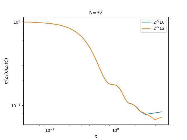
Now we can actually time evolve O for different trim values and plot the result:
# Time evolve O for different trim values
times = np.arange(0, 5 + 0.05, 0.05)
noise = 0.01
for trim in (10, 12):
    S = evolve(H, O, 2 ** trim, times, noise)
    plt.loglog(times, S, label=f"2^{trim}")

plt.legend()
plt.title(f"N={N}")
plt.xlabel("t")
plt.ylabel(r"$\mathrm{tr}(Z_1(0) Z_1(t))$")
plt.savefig("time_evolve_example.png")
plt.show()